Graph

Catalogue

1. 1. 1 图的计算机表示
   1. 1.1. Edge List
   2. 1.2. Adjacency Matrix
   3. 1.3. Adjacency List
   4. 1.4. Adjacency “Hash Set”
2. 2. 2 Graph Search Algorithm
   1. 2.1. Breadth First Search
      1. 2.1.1. Undirected Graph
      2. 2.1.2. Directed Graph
   2. 2.2. Dijkstra’s Algorithm
      1. 2.2.1. 743. Network Delay Time
      2. 2.2.2. 378. Kth Smallest Element in a Sorted Matrix
   3. 2.3. Depth First Search
      1. 2.3.1. Undirected Graph
      2. 2.3.2. Directed Graph
3. 3. 3 Application
   1. 3.1. 785. Is Graph Bipartite?
   2. 3.2. 133. Clone Graph

LeetCode 上很多问题都可以抽象成 “图” ，比如搜索类问题，树类问题，迷宫问题，矩阵路径问题，等等。Graph 是非常重要而又涵盖很广的内容，以至于有单独的”图论”研究方向。

1 图的计算机表示

1. Node / State
2. Edge / Action
3. Directed vs Undirected graph
4. Representation of the graph

Edge List

题目给的Nodes and Edges(Edge List)形式的图

• 要么考虑用Union Find，要么考虑重新建立图的表示

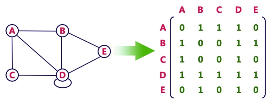
Adjacency Matrix

• Pros: Representation is easy to implement. Edge removal takes O(1) time. Queries like whether there is an edge from vertex ‘u’ to vertec ‘v’ are efficient and can be done O(1)
• Cons: Consumes more space O(V^2)(V is the number of vertex/node) Even if the graph is sparse(contains less number of edges) == waste of space

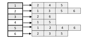
Adjacency List

Vertices/Nodes : V, Edges : E

• Pros: Space Complexity = O(V + E). Adding a vertex.node to the graph is easier
• Cons: Time Complexity is O(V) to check wheter there is an edge from a node to the other.(Comprared to O(1) in adjacent matrix)

Adjacency “Hash Set”

用hashset替代list表示相邻的节点，综合了Adjacency Matrix和Adjacency List的优点！

2 Graph Search Algorithm

Breadth First Search

How to describe a BFS’s action during an interview?

• Definition 1: expand a node s, 延展一个node
• Definition 2: generate s’s neighbor node: reach out to its neighboring node
• Data Structure : Maintain a FIFO queue, put all generated nodes in the queue
• Termination condition : do a loop until the queue is empty

Discussion

• When we deal with the tree-related problem and in the meantime we need to address the relationship on the same level
• BFS is NOT the right algorithm to find the shortest path in the graph
• BFS 的时间空间占用以 branching factor 为底, 到解的距离 d 为指数增长；
• BFS 空间占用上 Queue 是不会像 DFS 一样只存一条路径的，而是从起点出发越扩越大，因此会有空间不够的风险，空间占用为 O(b^d)。

Assume Input - graph adjacency “hash set”

Undirected Graph

• Queue, visited

# 其实和Tree的BFS traversal是一样的！
# Why visited array? 如果有环的话需要，没有环的话就是tree了，所以不需要！
def BFS1():
    visited = [0] * n
    queue = collections.deque([0])
    while queue:
        node = queue.popleft()
        print(node)
        visited[node] = 1
        for nei in graph[node]:
            if visited[nei] == 0:
                queue.append(nei)

Directed Graph

• Only directed graph has indegree and outdegree!

# 从Indegree == 0 的node开始！
def BFS2():
    queue = collections.deque([i for i in xrange(n) if indegree[i] == 0]）
    while queue:
        node = queue.popleft()
        print(node)
        for nei in graph[course]:
            indegree[nei] -= 1
            if indegree[nei] == 0:
                queue.append(nei)

Dijkstra’s Algorithm

“呆克斯戳” Best First Search, 也是BFS

1. Usages: Find the shortest path cost from a single node (source node) to any other nodes in that graph
2. Data Structure: Priority Queue (Min Heap)
3. Process

• Initial state (start node)
• Node expansion/ Generation rule
• Termination condition 所有点计算完毕也是”Queue is empty”

4. Properties

• One node can be expanded once and only once
• One node can be generated more than once. (cost can be reduced over time)
• all the cost of the nodes that are expanded are monotonically non-decreasing（所有从 priority queue里面pop出来的元素的值是单调非递减->单调递增）
• time complexity, for a graph with n node and the connectivity of the node is O(nlogn)
• when a node is popped out for expansion, its value is fixed which is equal to the shortest distance from the start node (非负权重)

743. Network Delay Time

class Solution(object):
  def networkDelayTime(self, times, N, K):
      graph = [[] for _ in xrange(N+1)]
      for u, v, w in times:
          graph[u].append((v, w))

      dis = [0] + [-1] * N  
      pq = [(0, K)]

      while pq:
          w, s = heapq.heappop(pq)
          if dis[s] >= 0:
              continue
          dis[s] = w
          for nxt, nw in graph[s]:
              heapq.heappush(pq, (w+nw, nxt))
      return -1 if -1 in dis else max(dis)

378. Kth Smallest Element in a Sorted Matrix

• Time : O(klogk), Space : O(k)

class Solution(object):
    def kthSmallest(self, matrix, k):
        n = len(matrix)
        visited = set([(0, 0)])
        heap = [(matrix[0][0], 0, 0)]

        for _ in xrange(k):
            val, x, y = heapq.heappop(heap)

            # next row
            if x+1 <= n-1 and (x+1, y) not in visited:
                heapq.heappush(heap, (matrix[x+1][y], x+1, y))
                visited.add((x+1,y))

            # next col
            if y+1 <= n-1 and (x, y+1) not in visited:
                heapq.heappush(heap, (matrix[x][y+1], x, y+1))
                visited.add((x,y+1))

        return val

Depth First Search

Backtracking is just a behavior of DFS

• DFS 的时间占用以 branching factor 为底，树的深度 m 为指数增长
• DFS 的空间占用上，却只是 O(bm)，可视化探索过程中只把每个 Node 的所有子节点存在 Stack 上， 探索完了再 pop 出来接着探，因此储存的节点数为 O(bm)。

可以看到无论是 BFS 还是 DFS，树的 branching factor 都是对空间与时间复杂度影响最大的参数；除此之外，BFS 中最重要的是到解的距离，而 DFS 看从当前节点的深度。普遍来讲，DFS 空间上会经济一些，当然也要分情况讨论。

Undirected Graph

def dfs(node):
    visited.add(node)
    for nei in node.neighbors:
        if nei not in visited:
            dfs(nei)

Directed Graph

• visited 需要 三种状态!!! 0-未访问，1-正在访问，2-已经访问

3 Application

785. Is Graph Bipartite?

• BFS的做法有一个问题，就是这个图可能不是连通图！！！所以要遍历所有点！
• 所有点有两次一次push进Queue，一次pop出Queue！

class Solution(object):
    def isBipartite(self, graph):
        n = len(graph)
        visited = [False] * n
        A, B = set(), set()
        for i in range(n):
            if visited[i]:
                continue

            queue = collections.deque([(i,0)])
            while queue:
                node, level = queue.popleft()

                if level:
                    B.add(node)
                else:
                    A.add(node)

                if visited[node]:
                    continue

                for nei in graph[node]:
                    queue.append((nei, 1 - level))
                visited[node] = True
        return not A&B

133. Clone Graph

克隆Graph，很多graph都是用HashTable一一映射

• Hash Table 新旧node一一映射，再把关系同样映射！
• DFS，BFS都可以把所有node遍历一遍就好

# BFS
class Solution:
    def cloneGraph(self, node):
        if not node:
            return None

        gmap = {node:UndirectedGraphNode(node.label)}
        queue = collections.deque([node])
        while queue:
            nnode = queue.popleft()
            for nei in nnode.neighbors:
                if nei not in gmap:
                    gmap[nei] = UndirectedGraphNode(nei.label)
                    queue.append(nei)
                gmap[nnode].neighbors.append(gmap[nei])
        return gmap[node]

# DFS
class Solution:
    def cloneGraph(self, node):
        return self.dfs(node, {})

    def dfs(self, node, cache):
        if not node:
            return None

        if node in cache:
            return cache[node]

        copy = UndirectedGraphNode(node.label)
        cache[node] = copy

        for nei in node.neighbors:
            nnei = self.dfs(nei, cache)
            copy.neighbors.append(nnei)
        return copy